¶ Submitting jobs
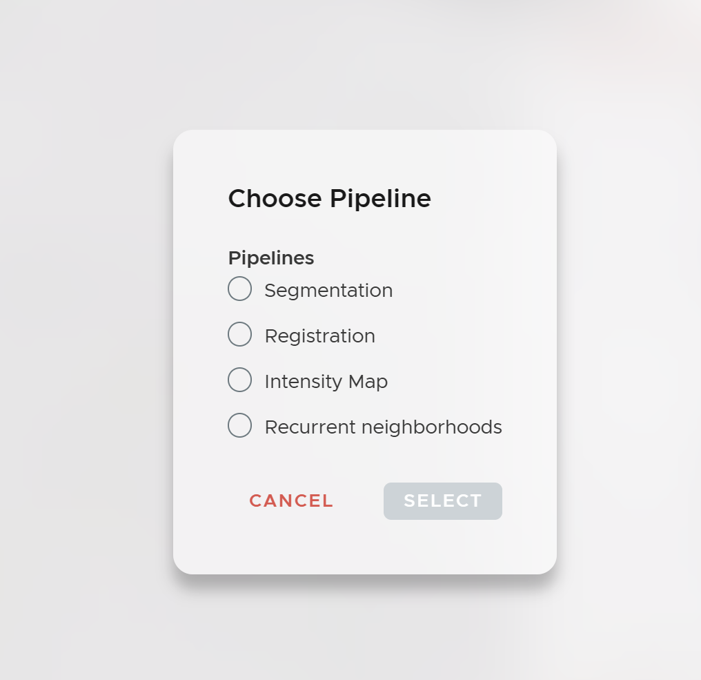
The essence of ariadne.ai SPATIAL is to provide a worry- and code-free analysis platform for spatial biology analysis. All analysis steps are packed into easily understandable jobs. To analyze your data, submit jobs in the order described below.
¶ Preprocessing
¶ Registration
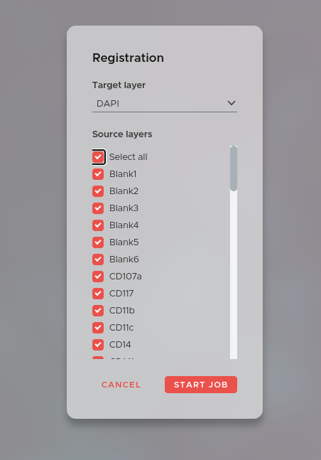
Registration is the first crucial preprocessing step to ensure best results during later analysis. Our elastic registration is scalable and highly precise.
To submit a registration job for your data click on the NEW JOB button in the main window and select Registration. The window above will open. Now select a target layer. This can be an H&E layer or for example the DAPI layer of your first staining cycle. Afterwards select all layers you want to register onto the target layer.
Always use the registered versions of your layers in all subsequent jobs.
¶ Cell Segmentation
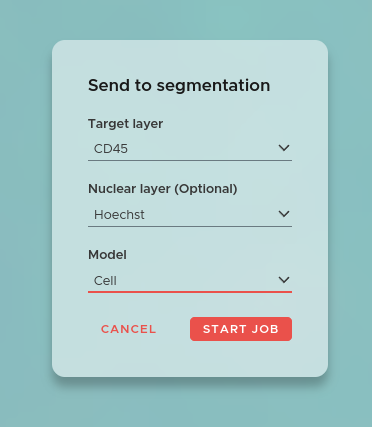
The essence of spatial biology is mapping the detections of omics markers to single cells or even smaller subcellular compartments. To achieve this, a very precise segmentation of the cells is necessary.
The segmentation in SPATIAL allows precise segmentation of histology data and fluorescence microscopy data in 2 and 3 dimensions. We even support highly complex cell types like neurons.
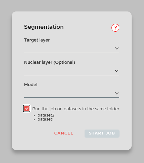
To start a segmentation job click on the NEW JOB button in the main window and select Segmentation. The window above will open. Now select the Target layer which will be used to perform the segmentation. Additionally, you can also choose to add a Nuclear layer, which will be used together with the target layer to improve segmentation accuracy.
¶ Nucleus Expansion
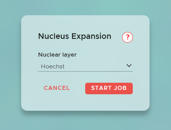
In a nucleus expansion job in SPATIAL, the process begins by segmenting the nuclei within the data. After segmentation, the algorithm expands these nuclear masks to cover the entire cell, achieving full cell segmentation.
This approach is particularly useful when only a nuclear marker (e.g. DAPI) is available and no membrane or cytoplasm channel exists.
To start, click NEW JOB and select Nucleus Expansion. Choose the Nuclear Layer to segment, and the algorithm will expand the nuclei to generate the complete cell segmentation.
¶ Intensity Map
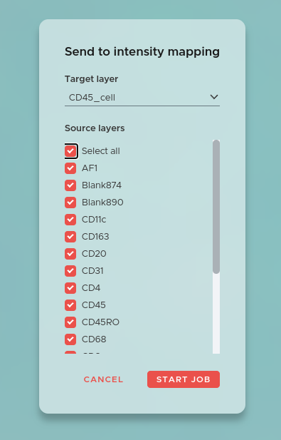
The Intensity Map job measures the expression of each marker within every segmented cell, creating the per-cell data table that all downstream statistical analysis depends on. In SPATIAL this per-cell table is called a Mapping. For more information on how to work with Mappings and their properties, see the Mappings & Properties page.
To start an Intensity Map job click on the NEW JOB button and select Intensity Map. Select a segmentation as the Target layer, onto which the marker intensities from all image channels will be mapped.
Optionally, select a Mask layer. If a mask is provided, only cells that overlap with the mask (for example a tissue region segmentation) will be included. Cells outside the mask are excluded from the Mapping. This is useful when you want to restrict your analysis to a specific tissue compartment.
¶ Dimensionality reduction
These jobs require a completed Intensity Map (Mapping) before they can be run.
¶ t-SNE

t-SNE (t-distributed Stochastic Neighbor Embedding) reduces the high-dimensional per-cell marker expression data to two dimensions, making it possible to visualize and explore cell populations in an interactive 2D scatter plot. Cells with similar marker profiles cluster together.
To start a t-SNE job click on the NEW JOB button and select t-SNE. Select the Mapping to use as input and choose which markers and morphometric features to include. Select a normalization method (per-marker z-score normalization is recommended to prevent high-intensity markers from dominating the result).
Set the algorithm parameters:
- Perplexity — controls the balance between local and global structure. Typical values are 5–50. Start with 30 if unsure.
- Number of iterations — more iterations improve convergence. 1000 is a good default; increase for large datasets.
- Learning rate — affects convergence speed. The default value is suitable for most datasets.
Give the experiment a name and submit. When the job completes, open the results in the right panel. The scatter plot is interactive: draw gates directly on the plot to define cell Selections.
¶ UMAP

UMAP (Uniform Manifold Approximation and Projection) is an alternative to t-SNE for dimensionality reduction. UMAP tends to better preserve the global structure of the data and is faster on large datasets.
To start a UMAP job click on the NEW JOB button and select UMAP. Select the Mapping and input features as for t-SNE, and set the normalization method.
Set the algorithm parameters:
- Number of neighbors — controls local vs. global structure preservation. Typical values are 5–50.
- Minimum distance — controls how tightly points are packed in the embedding. Values between 0.0 and 1.0; lower values produce more tightly packed clusters.
- Spread — works together with minimum distance to control cluster size.
- Distance metric — the metric used in the high-dimensional space. Euclidean is the default and works well for most marker expression data.
- Number of epochs — more epochs improve embedding quality at the cost of computation time.
Give the experiment a name and submit. Results are accessible in the right panel with the same interactive gating functionality as t-SNE.
¶ Cell type identification
¶ Automatic Cell Type Detection

Automatic Cell Type Detection (ACD) uses the per-cell marker expression data from a Mapping to automatically classify each cell into a predefined set of cell types. The classification is performed by a machine learning model trained on your marker panel.
To start an ACD job click on the NEW JOB button and select Automatic Cell Type Detection. Select the Mapping to use as input and choose the markers to include in the classification. Include all markers that are relevant to distinguishing the cell types of interest.
When the job completes, a new Categorical Property is added to your Mapping. Each cell receives a predicted cell type label. These labels are visible in the viewer as a color-coded overlay and can be used in all subsequent analysis steps — including Plotting, RCN, and Neighborhood Enrichment — as grouping variables.
¶ Spatial analysis
These jobs require both a completed Intensity Map (Mapping) and defined Selections.
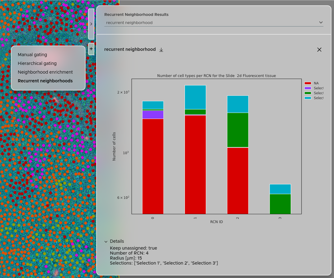
¶ Recurrent Neighborhoods
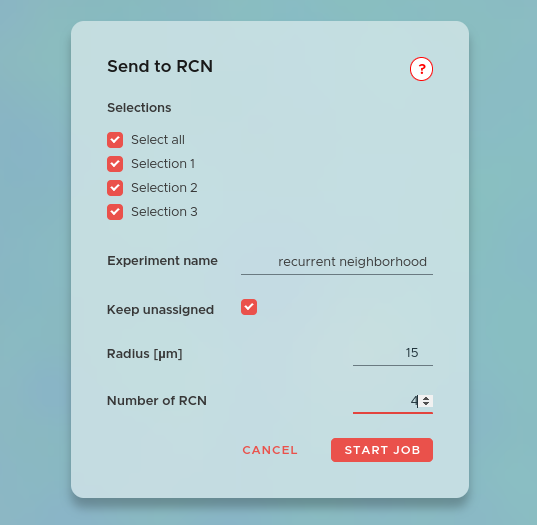
Recurrent cellular neighborhoods (RCN) identify recurring spatial microenvironments in your tissue based on the composition of cell types surrounding each cell. Each RCN represents a distinct pattern of cellular organization that repeats across the tissue section.
To start, click NEW JOB and select Recurrent Neighborhoods. Choose the selections you want to include in the RCN calculation. Both free selections (manually drawn gates) and hierarchical selections (structured groups, e.g. from ACD or UMAP gating) are supported. If your selections do not cover all cells but you want to keep them in the calculation, tick Keep unassigned — this groups unclassified cells under the name "NA" and treats them as a separate population. Then select a cutoff radius (all cells closer than this distance will be considered connected) and the number of RCNs to identify. A smaller number gives broader, coarser neighborhoods; a larger number yields finer, more specific microenvironments.
Give the experiment a name and submit. Each calculation can be reached via its Experiment Name.
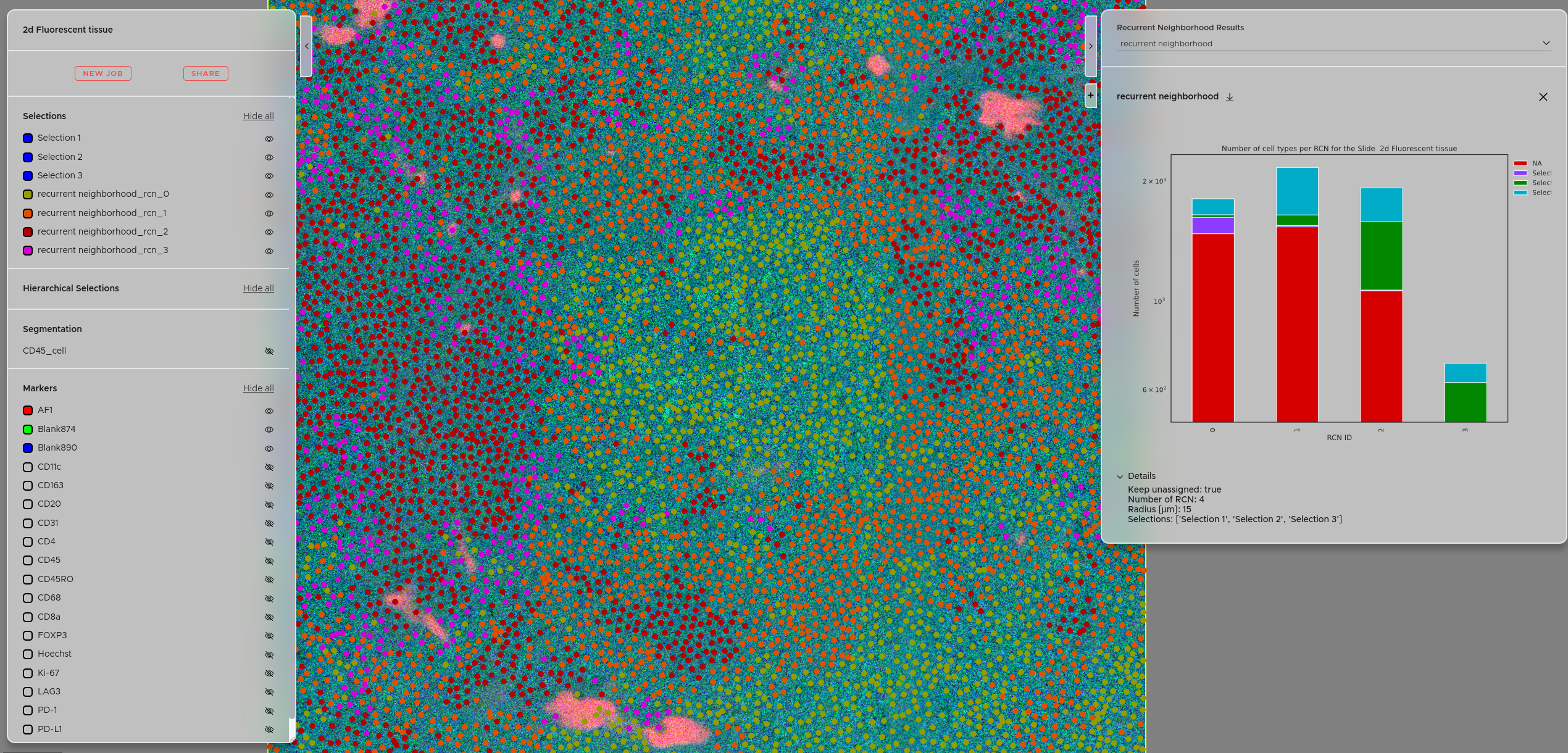
You can access the recurrent neighborhood results using the right panel → Click + → Select Recurrent neighborhoods. Your experiments will be accessible via the dropdown menu. The details of each experiment are accessible via the Details tab. You can also download the results as a zip file using the download button. The calculated recurrent neighborhoods will also be available under the "Selections" panel, letting you visualize exactly where each microenvironment occurs in the tissue.
For a detailed description of the RCN method, see the Statistical analysis page.
¶ Neighborhood Enrichment

The Neighborhood Enrichment score quantifies the pairwise spatial association between your defined cell populations. A positive score means two populations are found more often in each other's vicinity than expected by chance. A negative score means they tend to avoid each other spatially.
To start, click NEW JOB and select Neighborhood Enrichment. Choose the selections you want to include. Both free and hierarchical selections are supported. If your selections do not cover all cells but you want to include them in the computation, click Keep unassigned — this groups unclassified cells under the name "NA". This does not affect the enrichment score between any other selections. Then select the cutoff radius. All cells closer than this distance will be considered connected.
Give the experiment a name and submit.
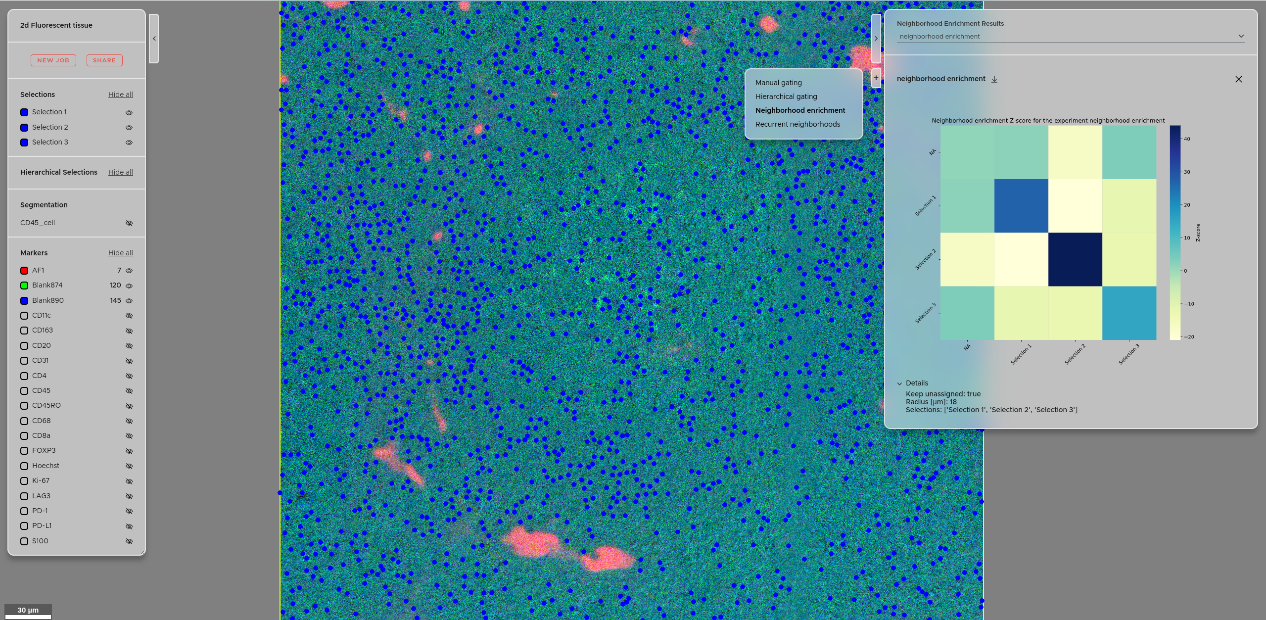
You can access the neighborhood enrichment score results using the right panel → Click + → Select Neighborhood enrichment. Your experiments will be accessible via the dropdown menu. The details of each experiment are accessible via the Details tab. You can also download the results as a zip file using the download button.
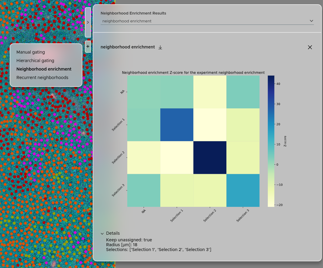
For a detailed description of the Neighborhood Enrichment method, see the Statistical analysis page.
¶ Visualization & reporting
¶ Plotting

The Plotting job generates statistical plots from your per-cell Mapping data, with support for cross-dataset comparisons using Cohorts. Two plot types are available:
- Box plot — displays the distribution of a single marker or feature across defined groups of cells.
- Heatmap — displays the expression of multiple markers across groups simultaneously, useful for comparing cell type signatures side by side.
Groups can be defined in three ways:
- Selections — groups cells by their membership in a named selection (e.g. a manually gated population or an ACD-defined cell type).
- Cohorts — groups datasets by the folder they belong to, enabling comparison across experimental conditions, patients, or time points.
- Categorical properties — groups cells by the value of a Categorical Property (e.g. tissue region type from a tissue segmentation).
To start, click NEW JOB and select Plotting. Select the Mapping to use as the data source and the plot type. Select the Property (marker or feature) to plot — for Heatmaps, multiple Properties can be selected. Define the groups, give the plot a name, and submit.
Before submitting a Plotting job that uses Cohorts, SPATIAL will warn you if any dataset in the cohort is missing the selected Mapping, Selections, or Properties. Review and resolve these warnings before submitting.
¶ Optional custom jobs (contact us)
¶ Add Mapping Property
You can extend an existing Mapping with new computed properties without rerunning the full Intensity Map job. The Add Mapping Property job computes new per-cell measurements by sampling additional marker layers within a defined radius around each cell, or by incorporating additional segmentation layers as spatial features. See the Mappings & Properties page for full details.
¶ Virtual marker segmentation
A precise cell segmentation might need not only one, but multiple markers. Get in touch with us to create a virtual marker combined of multiple markers, to get the best possible cell segmentation.
¶ Tissue segmentation
A tissue segmentation based on morphological features of the cells in your tissue provides you with a spatial marker independent tissue classification — giving you a great tool to find even subtle expression changes between different experiments. Depending on your tissue type the nuclei alone might be already sufficient. Contact us for a custom offer.
¶ Stitching
Precise stitching of your image tiles is more important than ever, especially when working with point-like signals like in spatial transcriptomics. We have multiple years of experience with image stitching and will deliver best results for your 2d or 3d tiles, with or without overlap.
¶ Artefact segmentation
Get rid of your imaging artefacts using our custom artefact segmentation. Common artefacts that we remove for our customers are air bubbles, fibers or hairs, dust particles and tissue folds.
¶ Ongoing jobs
To see your ongoing jobs click on the JOBS button in the navigation panel (top left).
¶ Submit batch jobs
You can apply the same job to multiple datasets at once. Note that the feature is only available if sibling datasets (within the same folder) exist.